


"Inflation is a disease," Friedman used to say—a disease that can only be cured by the central bank. Inflation surged but is now decelerating. Nevertheless, experiencing such a "disease" has been unfortunate, given its consequences on the population, particularly low-income households. This episode has brought dominant themes in macroeconomics back to the forefront and redirected central banks toward their primary and natural objective: maintaining a stable and low inflation rate.
In the work “It’s Baaack: The Surge in Inflation in the 2020s and the Return of the Non-Linear Phillips Curve”, with Gauti Eggertsson, we provide empirical and theoretical foundations for an inverse-L-shaped New Keynesian Phillips curve. This framework aligns with the evidence on inflation observed in the U.S. economy over the last 60 years.
Phillips (1958), in his seminal work, plotted data for U.K. wage inflation against the unemployment rate over a specific period. He showed a non-linear relationship between wage inflation and the unemployment rate. At low unemployment rates, employers bid up wages to attract workers, explaining the surge in wage inflation. Conversely, at high unemployment rates, workers are reluctant to accept wages below prevailing levels, leading to sluggish wage adjustments. His findings and subsequent research have had significant policy implications, sparking ongoing debates in macroeconomics. One key question has been whether a central bank can stimulate the economy by raising inflation. This view has been debated, challenged, refuted, and significantly refined, particularly by incorporating the critical role of expectations in shifting the Phillips curve.

Our analysis builds on the above figure, which plots U.S. CPI inflation against the log of the vacancy-to-unemployment ratio (denoted as θ) for the period 1960–2024, divided into four sub-periods. The plots are particularly intriguing for the periods 1960–1969 and 2009–2024, which clearly display a piecewise, positively sloped linear relationship between inflation and economic activity, as measured by θ.
When θ exceeds the unitary value—what we term the "Beveridge Threshold," corresponding to a log value of zero—the relationship becomes noticeably steeper. This phenomenon is evident only in the 1960–1969 and 2009–2024 sub-periods, during which labor market tightness was exceptionally high and consistently surpassed the Beveridge Threshold. The Beveridge Threshold represents a point of neutrality in the labor market, where the number of posted vacancies that firms seek to fill is exactly equal to the number of workers looking for a job.
We interpret the suggestive evidence above as uncovering what we label the Inverse-L New Keynesian Phillips Curve. It is well-known and widely accepted that scatter plots, such as the one shown in the figure above, can be interpreted as “equilibrium” points arising from the intersection of aggregate demand and supply curves. However, to clearly display an aggregate supply curve, the shocks must originate from demand. Conversely, to display an aggregate demand curve, the shocks must arise from supply.
By inspection, the data points—particularly those associated with the recent inflationary surge—appear more indicative of an aggregate supply relationship. The real challenge for proponents of the dominance of supply shocks lies in presenting evidence of an aggregate demand curve, which is typically downward-sloping, within the above picture.
In the first part of our paper, we provide a standard identification strategy to support the view that this represents an aggregate supply relationship.
The second part of our paper proposes the theoretical foundations for the Inverse-L New Keynesian Phillips Curve.
Three key novel features I will describe are crucial for characterizing the curve:
Marginal costs for firms depend on the wages of new hires rather than the average real wage.
The model incorporates an employment agency that posts vacancies and recruits workers, resulting in a flexible real wage positively related to the vacancy-to-unemployment ratio (θ).
The wages of new hires do not fall below the wages of existing workers.
Our starting point aligns with the New Keynesian framework, where firms face costly adjustments in price-setting behavior, resulting in an aggregate supply equation in which inflation depends on real marginal costs and next-period expected inflation.
A key feature of our framework is the distinction between two types of workers: those already attached to the firm with existing wages and those searching for a job who will eventually be either newly hired or remain unemployed. If existing and new of workers are perfect substitutes in production and the wages of new hires cannot fall below those of existing workers, firms will prioritize utilizing their existing workforce before turning to new hires. The critical novelty of our framework, compared to the standard New Keynesian model, lies in the determination of real marginal costs. Given the described setting, real marginal costs are determined by the real wages of new hires. Consequently, the aggregate supply equation takes the form:

This novel feature of our framework is crucial for ensuring the robustness of our analysis, particularly given that the average real wage—proxied, for example, by the Employment Cost Index—declined at the onset of the inflationary surge rather than rising. This pattern is not observed when using measures of wages specific to new hires.
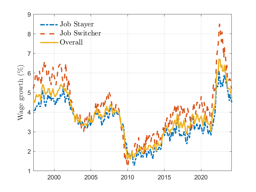
The figure below illustrates that the growth rate of nominal wages for job switchers, based on wage data from the Atlanta Fed Wage Tracker, has been significantly higher than that for job stayers. This is a distinctive characteristic of the latest inflationary episodes.
Labor-market search models, such as ours, are characterized by indeterminacy in the real wage. We address this issue by hypothesizing the presence of employment agencies that act on behalf of firms. These agencies post vacancies at a cost, facilitating appropriate matches between workers and firms, and benefit from the revenues corresponding to the wages of newly hired workers.
Using a standard matching technology, it follows that the equilibrium flexible real wage is proportional to the vacancy-to-unemployment ratio (θ), the variable we have identified as relevant in the figure above.
The flexible real wage is given by

In the above equation the gammas and η are parameters while “m” represents matching efficiency. To complete the model, and in the spirit of Phillips’s analysis, we assume that the wages of new hires align with the flexible wage determined above when the labor market is particularly tight. Conversely, when the labor market is loose, new hires will not accept wages below the prevailing levels. Therefore:

We model existing wages w^(ex) to adjust sluggishly, aligning closely with past wages while also responding mildly to market conditions, as proxied by the flexible wage. By incorporating all these elements into the Aggregate Supply equation described above, we derive the Inverse-L New Keynesian Phillips Curve:
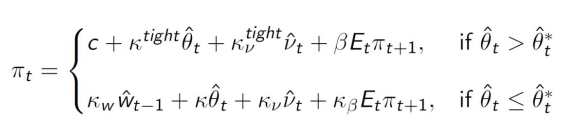
The Inverse-L New Keynesian Phillips Curve has a kink point at θ* above which labor market becomes tight, and below which the labor market is loose. This framework captures the relationship observed in the data while remaining consistent with the role of supply shocks as shifters, represented by the variable “v”, and with the influence of inflation expectations. A key feature of the model is that the coefficients κ^(tight) and κ_v^(tight), which apply in a tight labor market, are larger than the respective coefficients κ and κ_v, which apply in a loose labor market.
This distinction has two key implications:
Steeper Phillips Curve: When labor markets are tight (θ exceeds the Beveridge Threshold), the Phillips curve steepens in the inflation-θ diagram.
Amplified Supply Shocks: In tight labor markets, supply shocks have magnified effects on inflation, effectively "supercharging" their impact.

Our framework provides several key policy implications, as illustrated in the figure:
Demand Stimulus and Inflation: Post-COVID monetary and fiscal stimulus (shifting AD to AD′) would only modestly increase inflation if the Phillips curve were flat (E → E′′). However, under tight labor market conditions and a steep aggregate supply curve, demand stimulus can cause significant inflation, as seen in the U.S. recently.
Amplified Supply Shocks: Tight labor markets amplify supply shocks, shifting AS to AS′ and driving the economy from E to E′. This leads to higher inflation and an overheated economy.
Disinflation and Soft Landing: Contractionary monetary policy aimed at reducing AD predicts a mild impact on output, unemployment, and growth, supporting the feasibility of a soft landing—validated by recent U.S. economic trends.
References
Benigno, Pierpaolo and Gauti Eggertsson. 2024. It’s Baaack: The Surge in Inflation in the 2020s and the Return of the Non-Linear Phillips Curve. Unpublished Manuscript.